Backend.AI FastTrack 2 Guide for Airflow Users: Seamless Integration from Training to Serving

Engineering

ON THIS PAGE

Jun 29, 2025

Engineering

Backend.AI FastTrack 2 Guide for Airflow Users: Seamless Integration from Training to Serving

Jeongseok Kang
Researcher

Jun 29, 2025

Engineering

Backend.AI FastTrack 2 Guide for Airflow Users: Seamless Integration from Training to Serving

Jeongseok Kang
Researcher

Why Do We Need Backend.AI FastTrack 2?

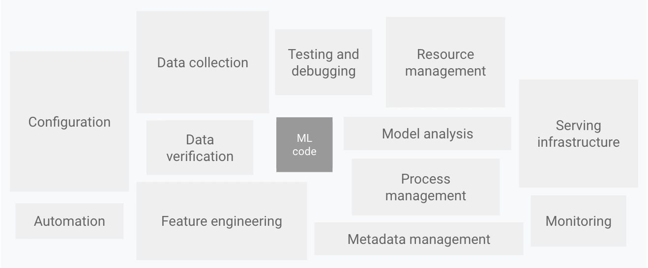
According to a 2014 Google paper, machine learning systems inherently contain significant technical debt, and the code responsible for training and inference represents only a small fraction of the overall system. The majority of the code is dedicated to integrating various components, not just the core ML logic¹².

Reality: ML Code Is Just the Tip of the Iceberg

Source: Google Cloud - MLOps: Continuous delivery and automation pipelines in machine learning

The actual machine learning code is merely the visible part of a much larger iceberg, while the rest consists of infrastructure, monitoring, and data pipeline engineering. As a result, managing these dependencies and enabling systematic experimentation, monitoring, and alerting through robust MLOps pipelines is becoming increasingly important.

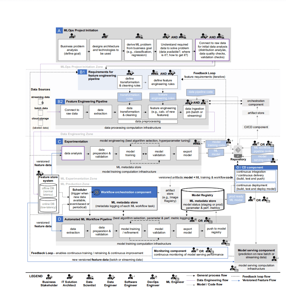Source: Machine Learning Operations (MLOps): Overview, Definition, and Architecture

Limitations of Existing MLOps Tools

A 2023 review paper³ highlights that while open-source projects like Airflow⁴ and Kubeflow⁵ are widely used, each has its own limitations:

Airflow: Excellent for workflow orchestration, but requires additional setup for GPU resource management and model serving.
Kubeflow: Powerful, but demands deep Kubernetes expertise and complex configuration.
Other tools: Often specialized for certain tasks, lacking an integrated user experience.

The Core Problem: Fragmented ML Workflows

Researchers and engineers face several challenges:

Complex infrastructure setup: Even simple model training often requires configuring Docker, Kubernetes, environment variables, and more.
Difficulty managing GPU resources: Efficient allocation and management of expensive GPU resources is challenging.
Complexity of model serving: Deploying trained models as production services requires separate tools and configurations.
Fragmented workflows: Different tools and platforms are used for each stage—training, validation, and serving—leading to inefficiencies.

The Solution: Backend.AI FastTrack 2 Model Serving

To address these challenges, Backend.AI has introduced an integrated model serving feature, as previously announced on our blog. With Backend.AI FastTrack 2, users can now leverage built-in model serving capabilities, enabling more efficient AI model deployment and management.

What is Model Serving? Model serving is the process of deploying a trained ML model as an API endpoint in a production environment, enabling real-time inference requests. This is the crucial step that transforms a model into real business value.

By integrating this feature, Backend.AI FastTrack 2 offers the following competitive advantages:

✅ End-to-end pipeline: Seamless workflow from model training and validation to serving.
✅ GPU resource optimization: Automatic scaling and efficient GPU allocation.
✅ Ready-to-use APIs: REST API endpoints are available immediately after training.
✅ Intuitive UI: Manage all tasks through a web interface.

Source: Backend.AI Architecture

A True Ally for Researchers

Backend.AI FastTrack 2 allows researchers to focus on core research without getting bogged down by infrastructure complexity. There’s no longer any need to waste time on Docker configuration, Kubernetes management, or writing complex deployment scripts.

Real-World Example: Migrating from Airflow to Backend.AI FastTrack 2

In this blog, we’ll use the MNIST (Modified National Institute of Standards and Technology) classification problem as an example to demonstrate how a pipeline previously managed with Airflow can be set up more simply and efficiently with Backend.AI FastTrack 2.

Pre- and Post-Migration Comparison

Category	Airflow	Backend.AI FastTrack 2
Setup Complexity	Docker Compose, environment variables, dependency management	A few clicks in the WebUI
GPU Management	Manual configuration required	Automatic allocation and optimization
Model Serving	Requires separate tools (FastAPI, Gradio, etc.)	Integrated serving functionality
Operational Costs	High (complex infrastructure management)	Low (optimized resource usage)

Airflow

Apache Airflow (hereafter Airflow) is an open-source workflow orchestration platform developed by Airbnb in 2014. It allows users to define and schedule complex data pipelines using Python code, which has led to its widespread adoption across many organizations.

The examples in this post use Airflow 3.0.2

In this blog, we’ll run Airflow using the official Docker image. If you’re not familiar with Docker environments, refer to the official Airflow documentation for detailed instructions.

Initial Airflow Setup

To use Airflow, you need several configuration files. Let’s walk through the setup process using a practical example.

[core]  # https://airflow.apache.org/docs/apache-airflow/stable/configurations-ref.html#core
auth_manager=airflow.api_fastapi.auth.managers.simple.simple_auth_manager.SimpleAuthManager
simple_auth_manager_users = admin:admin,user:user
simple_auth_manager_passwords_file = ./passwords.json
dags_folder = /opt/airflow/dags

[api]  # https://airflow.apache.org/docs/apache-airflow/stable/configurations-ref.html#api
host=0.0.0.0
port=8080

[api_auth]  # https://airflow.apache.org/docs/apache-airflow/stable/configurations-ref.html#api-auth
jwt_secret={JWT_SECRET_KEY}

[secrets]
backend = airflow.secrets.local_filesystem.LocalFilesystemBackend

PYTHONPATH=/opt/airflow/dags:$PYTHONPATH airflow standalone

services:
  airflow:
    image: apache/airflow:3.0.2-python3.12
    ports:
      - 8080:8080
    environment:
      AIRFLOW_HOME: /opt/airflow
    volumes:
      - .:/opt/airflow
      - ./dags/mnist/v1/.env:/opt/airflow/dags/mnist/v1/.env:ro
    entrypoint: /opt/airflow/compose/entrypoint.sh

Running and Initializing the Container

# Start Docker containers
$ docker compose -f docker-compose.yaml up -d

# Initialize (or reset) the database
$ docker exec -it <container_id> airflow db reset -y

Now, you can access Airflow at the default address(http://127.0.0.1:8080)Log in using the credentials generated in passwords.json:

{"admin": "7PdAaKvPb3E3fasz", "user": "USmGxuNAvvCRuyYs"}

Airflow - Login Screen

After logging in, click the Dags menu on the left to see that the DAG list is currently empty.

Airflow - DAG List Screen

Creating a DAG

In Airflow, a DAG (Directed Acyclic Graph) is defined using Python code. Let’s create a DAG that downloads the MNIST dataset and performs model training.

import os
from datetime import datetime, timedelta, timezone

from airflow.providers.standard.operators.python import PythonVirtualenvOperator
from airflow.sdk import DAG

HF_TOKEN = os.getenv("HF_TOKEN")

with DAG(
    dag_id="mnist",
    default_args={
        "depends_on_past": False,
        "retries": 1,
        "retry_delay": timedelta(minutes=5),
    },
    description="PyTorch MNIST classifcation example DAG",
    params={
        "hf_token": HF_TOKEN,
    },
    start_date=datetime.now(timezone.utc) + timedelta(seconds=10),
    catchup=False,
    tags=["example"],
) as dag:
    def download_mnist_dataset(**kwargs) -> None:
        import os
        from pathlib import Path

        import datasets

        AIRFLOW_HOME = os.getenv("AIRFLOW_HOME", "/opt/airflow")
        dataset_path = Path(AIRFLOW_HOME) / "datasets" / "mnist"
        if not dataset_path.exists():
            dataset_path.mkdir(parents=True, exist_ok=True)

        dataset = datasets.load_dataset(
            "ylecun/mnist",
            token=kwargs.get("hf_token"),
        )
        dataset.save_to_disk(dataset_path)

    download_mnist_dataset_task = PythonVirtualenvOperator(
        task_id="download_mnist_dataset",
        python_callable=download_mnist_dataset,
        requirements=["datasets"],
        system_site_packages=False,
        op_kwargs={
            "params": {
                "hf_token": dag.params.get("hf_token"),
            },
        },
    )

    def train_mnist_model(**kwargs) -> None:
        import os
        from pathlib import Path

        import torch
        import torch.optim as optim
        from torchvision import datasets, transforms
        from torch.optim.lr_scheduler import StepLR

        from mnist.v1.models import Net
        from mnist.v1.trainer import Trainer

        AIRFLOW_HOME = os.getenv("AIRFLOW_HOME", "/opt/airflow")
        dataset_path = Path(AIRFLOW_HOME) / "datasets" / "mnist"

        use_accel = not kwargs["params"]["no_accel"] and torch.accelerator.is_available()

        torch.manual_seed(kwargs["params"]["seed"])

        if use_accel:
            device = torch.accelerator.current_accelerator()
        else:
            device = torch.device("cpu")

        train_kwargs = {"batch_size": kwargs["params"]["batch_size"]}
        test_kwargs = {"batch_size": kwargs["params"]["test_batch_size"]}
        if use_accel:
            accel_kwargs = {
                "num_workers": 1,
                "pin_memory": True,
                "shuffle": True,
            }
            train_kwargs.update(accel_kwargs)
            test_kwargs.update(accel_kwargs)

        transform = transforms.Compose([
            transforms.ToTensor(),
            transforms.Normalize((0.1307,), (0.3081,))
        ])
        dataset1 = datasets.MNIST(dataset_path, train=True, download=True, transform=transform)
        dataset2 = datasets.MNIST(dataset_path, train=False, transform=transform)
        train_loader = torch.utils.data.DataLoader(dataset1, **train_kwargs)
        test_loader = torch.utils.data.DataLoader(dataset2, **test_kwargs)

        model = Net().to(device)
        optimizer = optim.Adadelta(model.parameters(), lr=kwargs["params"]["lr"])
        scheduler = StepLR(optimizer, step_size=1, gamma=kwargs["params"]["gamma"])

        trainer = Trainer(model)

        class AttributeDict(dict):
            def __getattr__(self, item):
                return self[item]

        for epoch in range(1, kwargs["params"]["epochs"] + 1):
            trainer.train(AttributeDict(kwargs["params"]), device, train_loader, optimizer, epoch)
            trainer.test(device, test_loader)
            scheduler.step()

        if kwargs["params"]["save_model"]:
            torch.save(model.state_dict(), "mnist_cnn.ckpt")

    train_mnist_model_task = PythonVirtualenvOperator(
        task_id="train_mnist_model",
        python_callable=train_mnist_model,
        requirements=["torch", "torchvision"],
        system_site_packages=False,
        op_kwargs={
            "params": {
                "lr": 1.0,
                "epochs": 14,
                "batch_size": 64,
                "test_batch_size": 1000,
                "gamma": 0.7,
                "no_accel": False,
                "dry_run": False,
                "seed": 1,
                "log_interval": 10,
                "save_model": True,
            },
        },
    )

    download_mnist_dataset_task >> train_mnist_model_task

import torch
import torch.nn as nn
import torch.nn.functional as F


class Net(nn.Module):
    def __init__(self):
        super(Net, self).__init__()
        self.conv1 = nn.Conv2d(1, 32, 3, 1)
        self.conv2 = nn.Conv2d(32, 64, 3, 1)
        self.dropout1 = nn.Dropout(0.25)
        self.dropout2 = nn.Dropout(0.5)
        self.fc1 = nn.Linear(9216, 128)
        self.fc2 = nn.Linear(128, 10)

    def forward(self, x):
        x = self.conv1(x)
        x = F.relu(x)
        x = self.conv2(x)
        x = F.relu(x)
        x = F.max_pool2d(x, 2)
        x = self.dropout1(x)
        x = torch.flatten(x, 1)
        x = self.fc1(x)
        x = F.relu(x)
        x = self.dropout2(x)
        x = self.fc2(x)
        output = F.log_softmax(x, dim=1)
        return output

import torch
import torch.nn.functional as F
import torch.optim as optim


class Trainer:
    def __init__(self, model: torch.nn.Module) -> None:
        self._model = model

    def train(
        self,
        args,
        device: torch.device,
        train_loader: torch.utils.data.DataLoader,
        optimizer: optim.Optimizer,
        epoch: int,
    ) -> None:
        self._model.train()
        for batch_idx, (data, target) in enumerate(train_loader):
            data, target = data.to(device), target.to(device)
            optimizer.zero_grad()
            output = self._model(data)
            loss = F.nll_loss(output, target)
            loss.backward()
            optimizer.step()
            if batch_idx % args.log_interval == 0:
                print("Train Epoch: {} [{}/{} ({:.0f}%)]\tLoss: {:.6f}".format(
                    epoch,
                    batch_idx * len(data),
                    len(train_loader.dataset),
                    100. * batch_idx / len(train_loader),
                    loss.item(),
                ))
                if args.dry_run:
                    break

    def test(
        self,
        device: torch.device,
        test_loader: torch.utils.data.DataLoader,
    ) -> None:
        self._model.eval()
        test_loss = 0
        correct = 0
        with torch.no_grad():
            for data, target in test_loader:
                data, target = data.to(device), target.to(device)
                output = self._model(data)
                test_loss += F.nll_loss(output, target, reduction="sum").item()
                pred = output.argmax(dim=1, keepdim=True)
                correct += pred.eq(target.view_as(pred)).sum().item()

        test_loss /= len(test_loader.dataset)

        print("\nTest set: Average loss: {:.4f}, Accuracy: {}/{} ({:.0f}%)\n".format(
            test_loss,
            correct,
            len(test_loader.dataset),
            100. * correct / len(test_loader.dataset),
        ))

Then run the DAG script you created to register with Airflow.

$ docker exec -it <container_id> python dags/mnist/v1/dag.py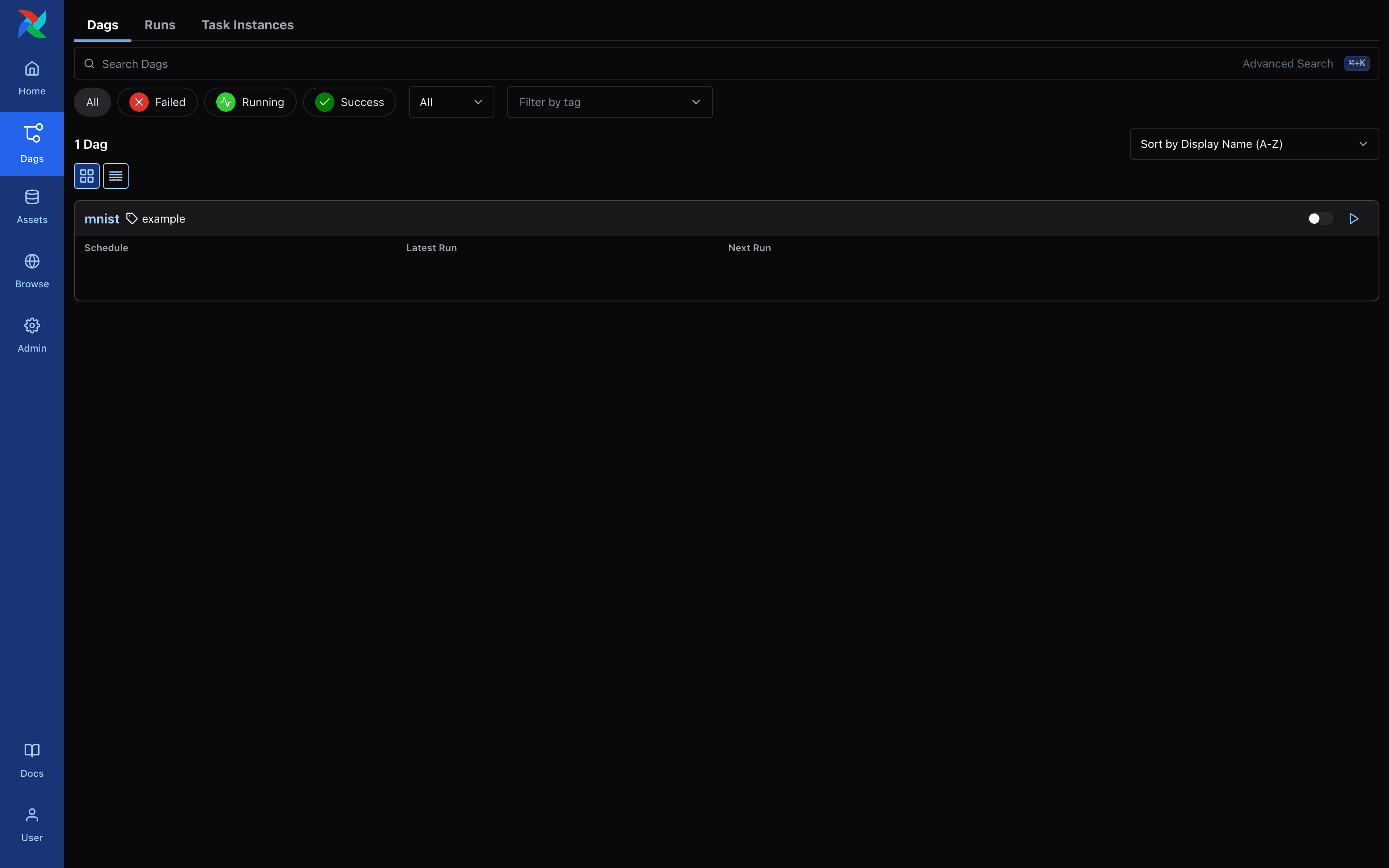

Airflow - DAG List Screen

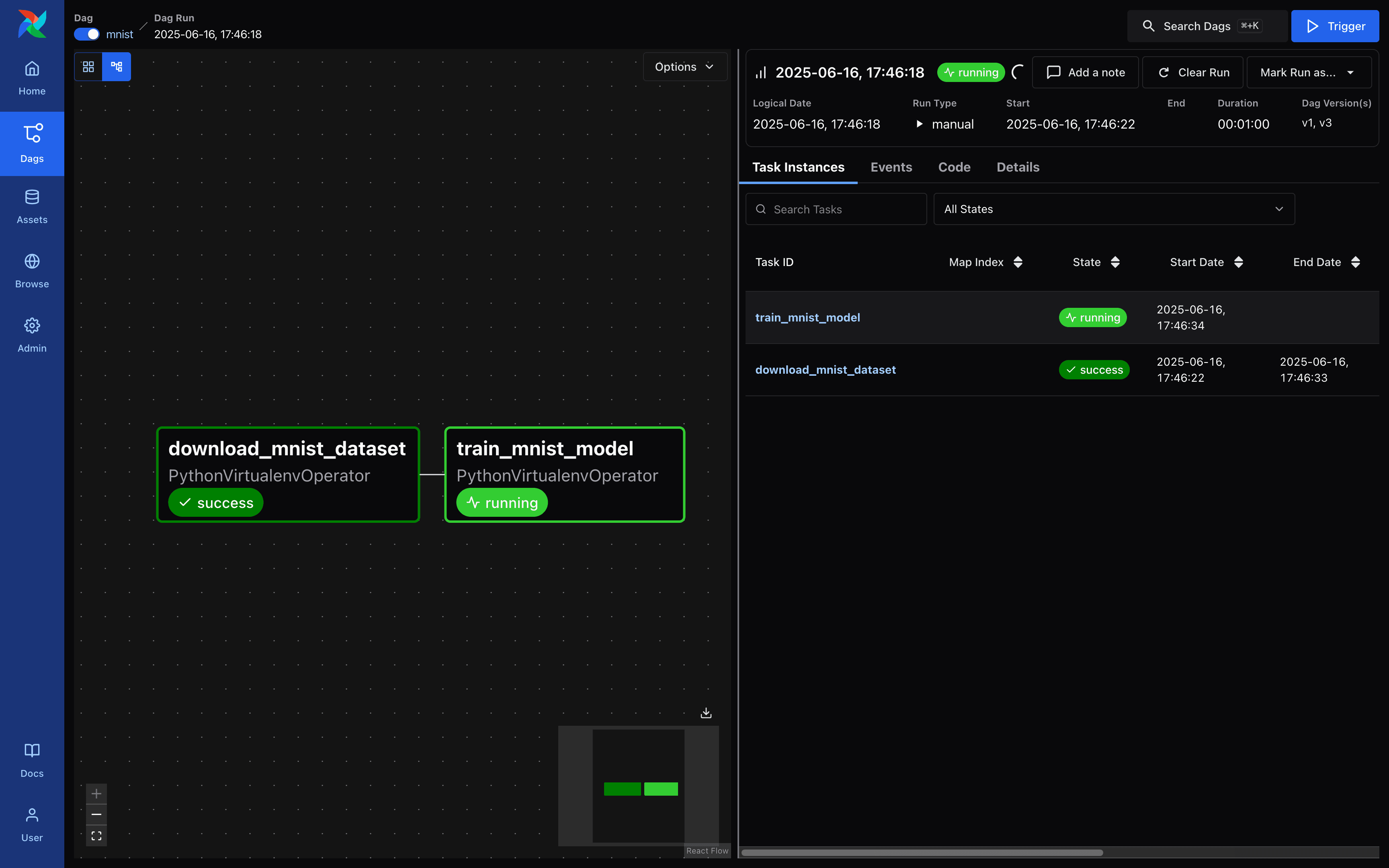
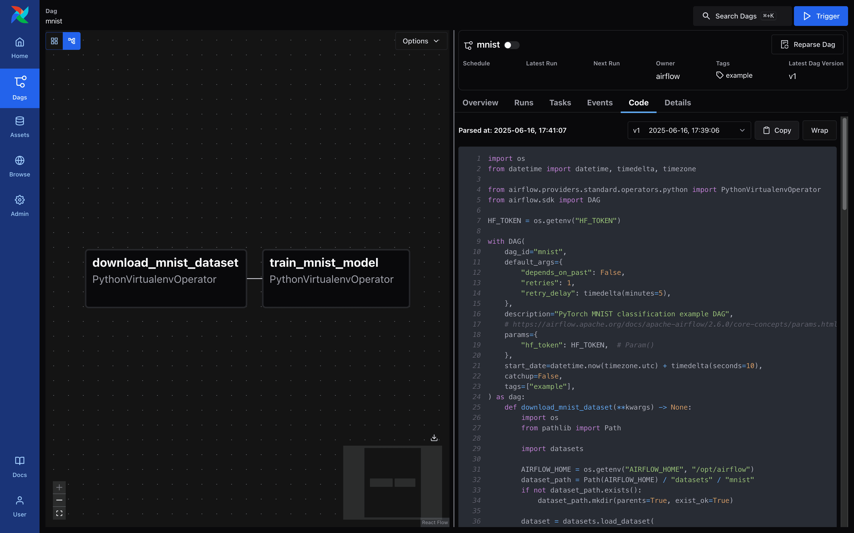Airflow - DAG Details Screen

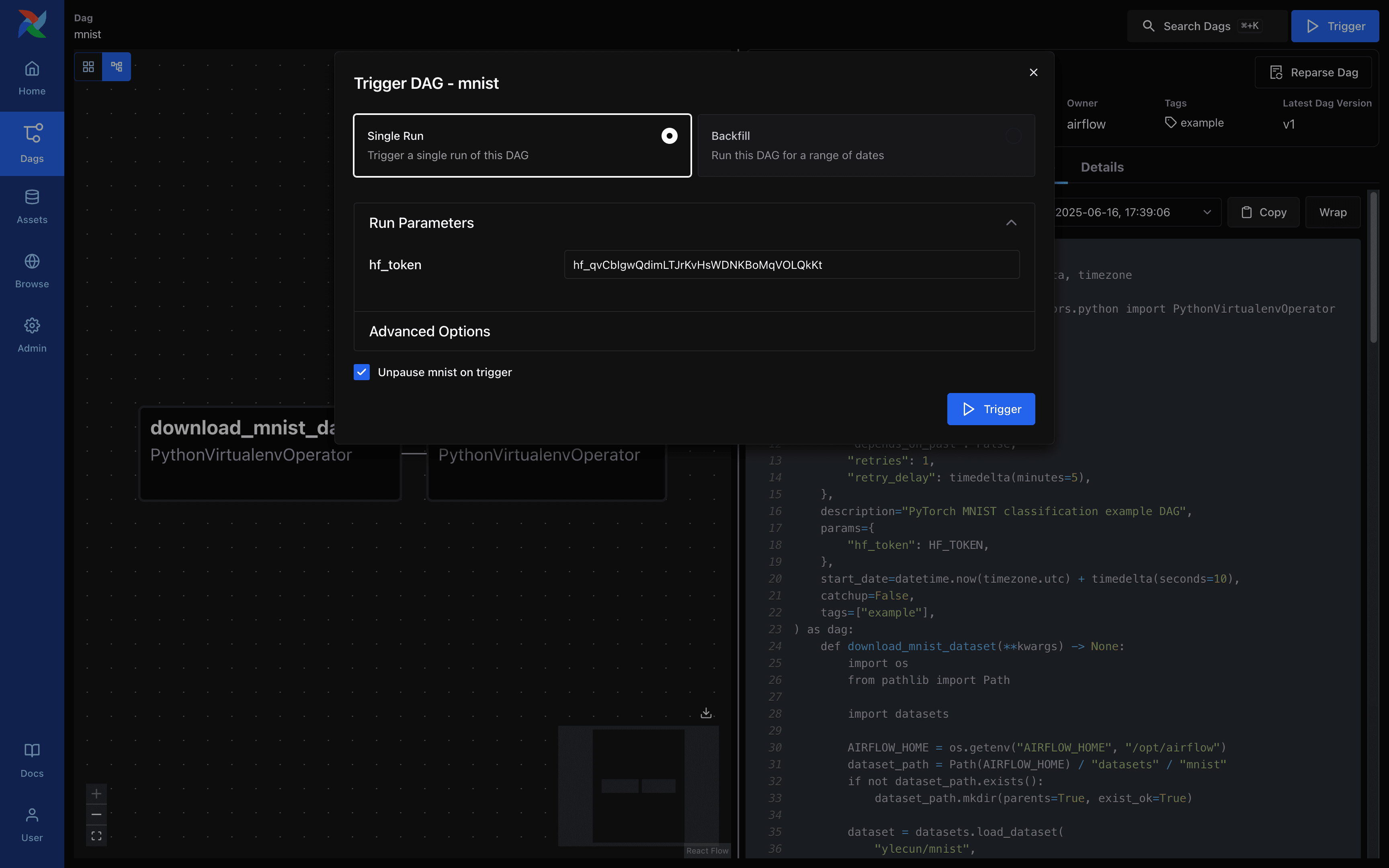Airflow - DAG Run Request Screen

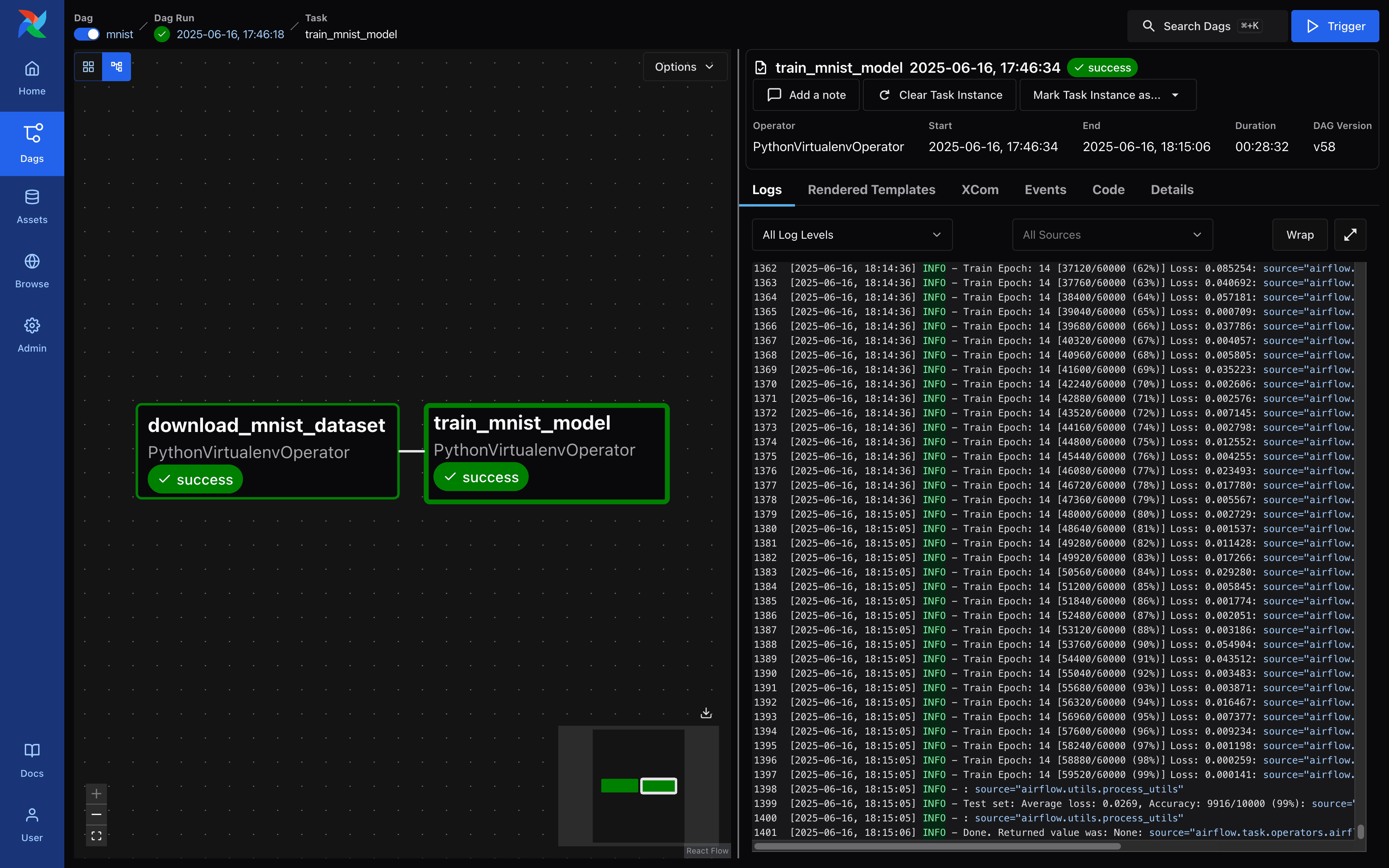
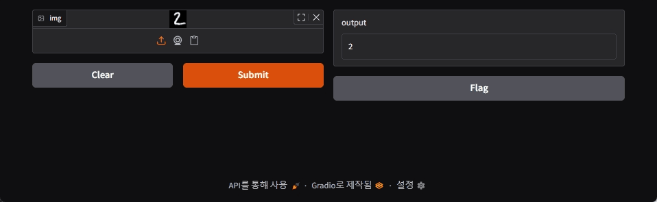
When the model is finished training, you can see that the file mnist_cnn.ckpt has been created. Next, create and run a simple Gradio demo to experiment with the MNIST model, as shown below.

$ pip install fastapi==0.115.12 gradio==5.33.0 torch==2.7.1 torchvision==0.22.1

from http import HTTPStatus
from pathlib import Path

import gradio
import numpy as np
import torch
from fastapi import FastAPI, Response
from fastapi.responses import JSONResponse
from torchvision import transforms

from models import Net

model = Net()
model.load_state_dict(torch.load(Path(__file__).parent.parent.parent / "mnist_cnn.ckpt"))

transform = transforms.Compose([
    transforms.ToTensor(),
    transforms.Normalize((0.1307,), (0.3081,)),
    transforms.Grayscale(),
])

app = FastAPI()


@app.get("/health", status_code=HTTPStatus.OK)
async def health_check() -> Response:
    return JSONResponse({"healthy": True})


def fn(img: np.ndarray) -> int:
    x = transform(img).unsqueeze(0)
    x = model(x)
    x = x.argmax(dim=1, keepdim=True)
    return int(x.item())


gradio_app = gradio.Interface(
    fn=fn,
    inputs=["image"],
    outputs=["number"],
)

app = gradio.mount_gradio_app(app, gradio_app, path="/")

$ fastapi run model-defs/gradio/main.py

   FastAPI   Starting production server 🚀
 
             Searching for package file structure from directories with __init__.py files
             Importing from /Users/rapsealk/Desktop/git/airflow-demo/model-defs/gradio
 
    module   🐍 main.py
 
      code   Importing the FastAPI app object from the module with the following code:
 
             from main import app
 
       app   Using import string: main:app
 
    server   Server started at http://0.0.0.0:8000
    server   Documentation at http://0.0.0.0:8000/docs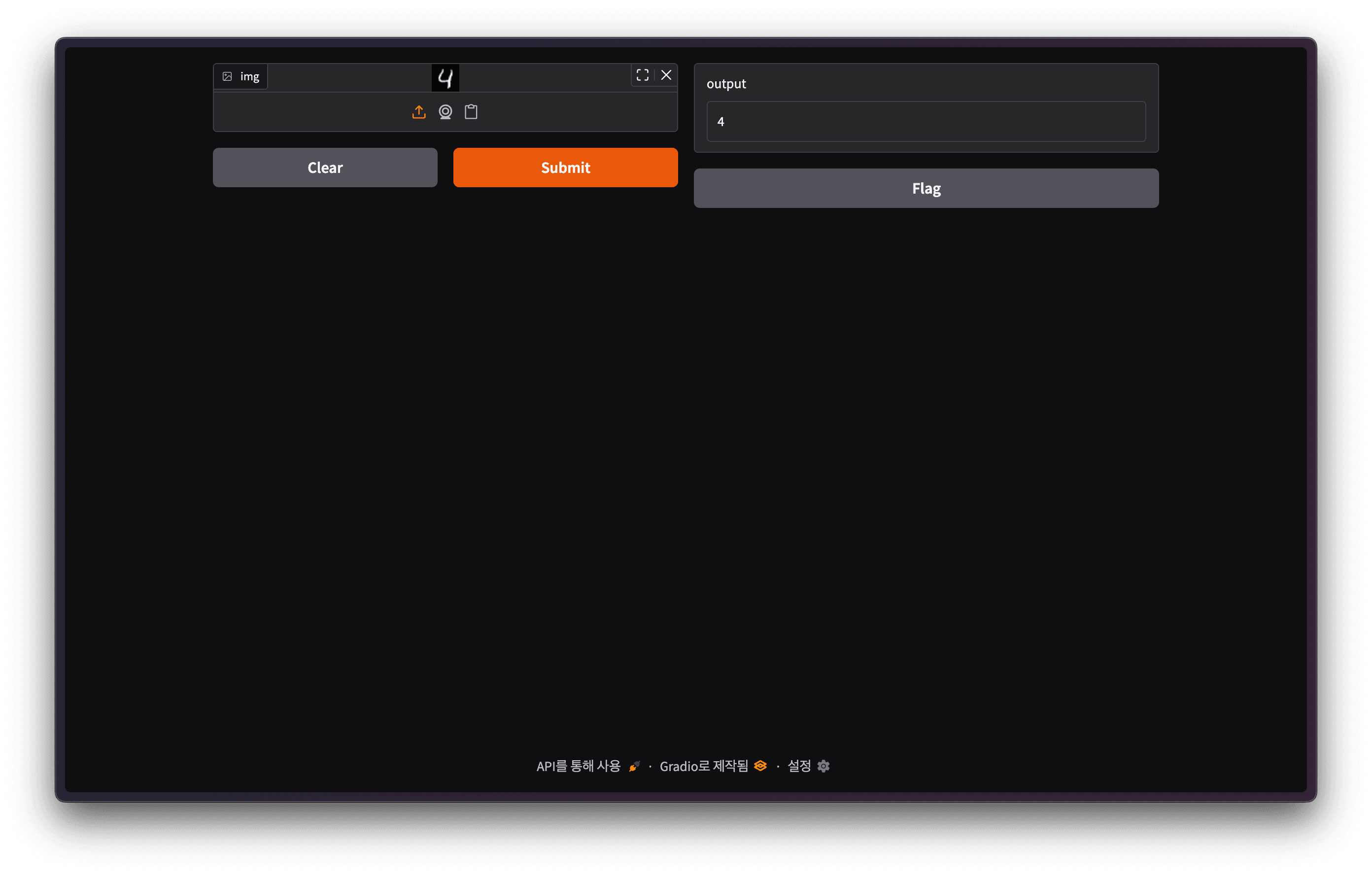

Gradio Demo Screen

Backend.AI FastTrack 2

This time, we will use Backend.AI FastTrack 2 to build the MNIST training and deployment pipeline. If you are not familiar with the Backend.AI FastTrack 2 pipeline, please refer to our previous blog.

NOTE

The examples contained herein were created using Backend.AI FastTrack 2 v25.9.0.

Connect to Backend.AI FastTrack 2 and click the Sign in button. You can access Backend.AI FastTrack 2 through your Backend.AI account.

Backend.AI FastTrack 2 Login Screen

Backend.AI Login Screen

Backend.AI FastTrack 2 Main Screen

Creating a new pipeline

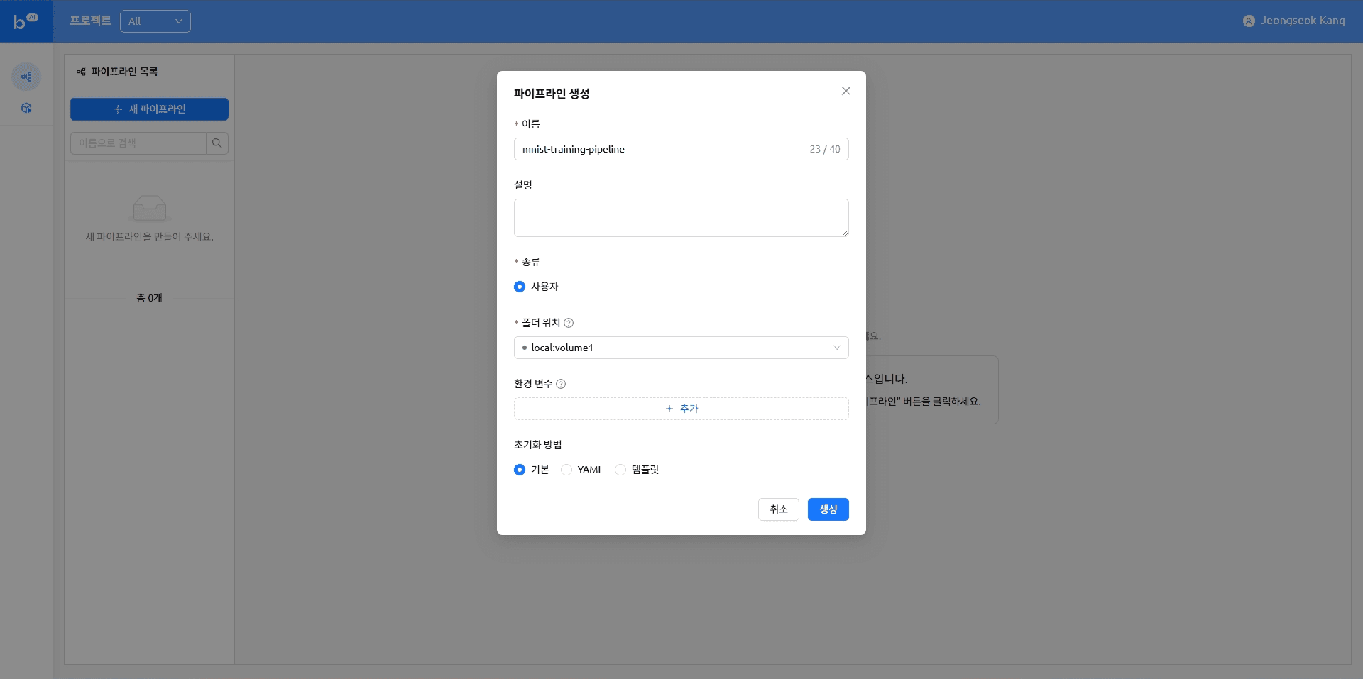
Uploading a file

The pipeline we are creating is designed to run a Python script stored in a VFolder. This table of contents covers how to upload the files needed to run the pipeline.

On the Backend.AI main screen, click the ‘Data’ item in the left menu.

Backend.AI Main

As you create the pipeline, you can see the pipeline folder that was created. Click a pipeline folder and upload a file.

VFolder List

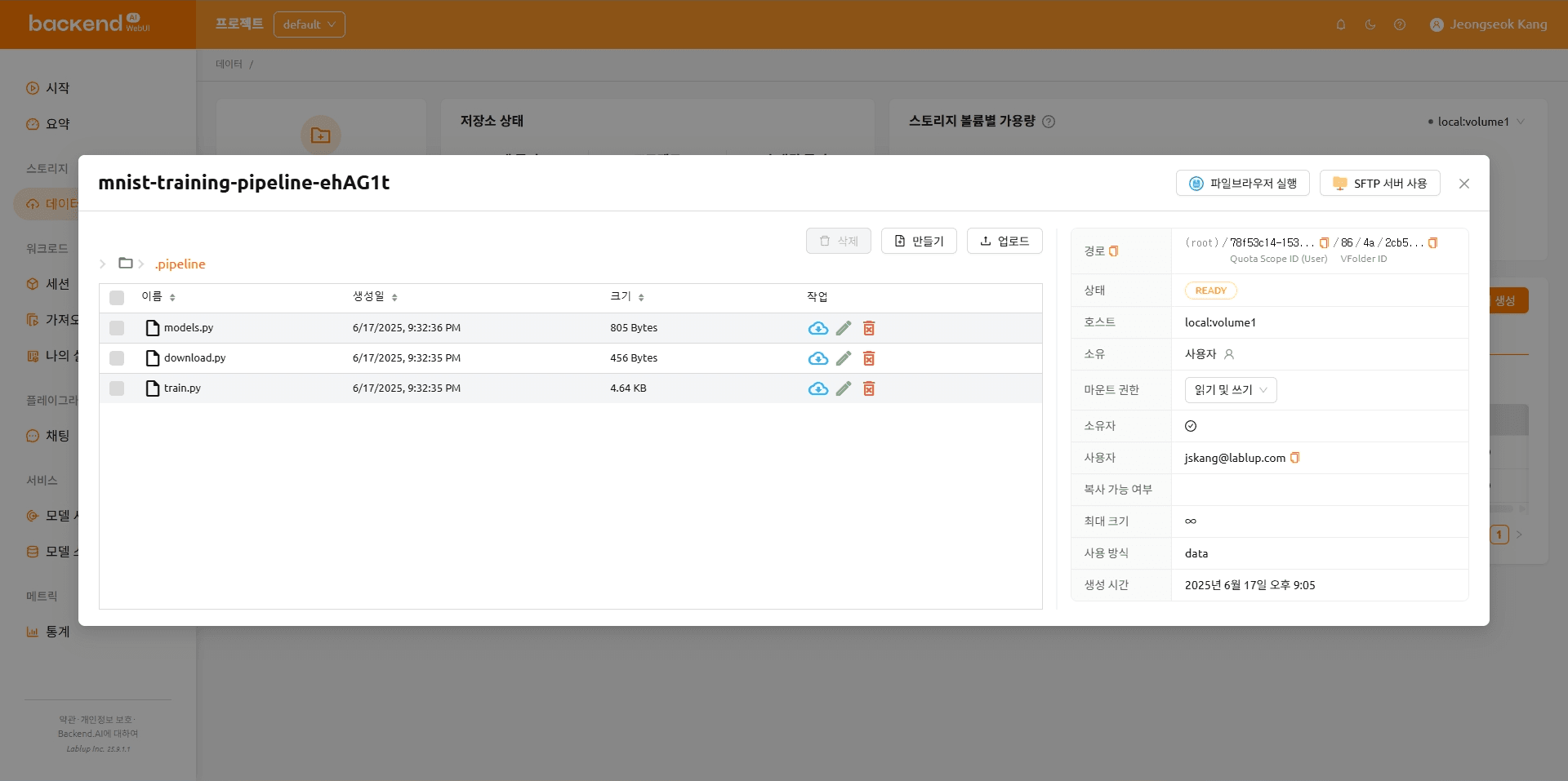The folder after the file upload is complete

The folder organization after the files are uploaded is shown below.

mnist-training-pipeline-ehAG1t
    |---- .pipeline
        |---- model.py
        |---- download.py
        \---- train.py

import torch
import torch.nn as nn
import torch.nn.functional as F


class Net(nn.Module):
    def __init__(self):
        super(Net, self).__init__()
        self.conv1 = nn.Conv2d(1, 32, 3, 1)
        self.conv2 = nn.Conv2d(32, 64, 3, 1)
        self.dropout1 = nn.Dropout(0.25)
        self.dropout2 = nn.Dropout(0.5)
        self.fc1 = nn.Linear(9216, 128)
        self.fc2 = nn.Linear(128, 10)

    def forward(self, x):
        x = self.conv1(x)
        x = F.relu(x)
        x = self.conv2(x)
        x = F.relu(x)
        x = F.max_pool2d(x, 2)
        x = self.dropout1(x)
        x = torch.flatten(x, 1)
        x = self.fc1(x)
        x = F.relu(x)
        x = self.dropout2(x)
        x = self.fc2(x)
        output = F.log_softmax(x, dim=1)
        return output

import os
from pathlib import Path

from torchvision import datasets

MNIST_DATASET_PATH = Path("/pipeline/vfroot") / os.getenv("MNIST_DATASET_PATH", "")


def main() -> None:
    train_dataset = datasets.MNIST(MNIST_DATASET_PATH, train=True, download=True)
    print(f"Train dataset is saved at: {train_dataset}")
    test_dataset = datasets.MNIST(MNIST_DATASET_PATH, train=False, download=True)
    print(f"Test dataset is saved at: {test_dataset}")


if __name__ == "__main__":
    main()

import argparse

import os
from pathlib import Path

import torch
import torch.nn.functional as F
import torch.optim as optim
from torchvision import datasets, transforms
from torch.optim.lr_scheduler import StepLR

from models import Net

MNIST_DATASET_PATH = Path("/pipeline/vfroot") / os.getenv("MNIST_DATASET_PATH", "")
CHECKPOINT_PATH = Path(os.getenv("CHECKPOINT_PATH")).joinpath(os.getenv("BACKENDAI_PIPELINE_JOB_ID", "mnist_cnn")).with_suffix(".ckpt")


def parse_args():
    parser = argparse.ArgumentParser(description="Train MNIST model")
    parser.add_argument("--lr", type=float, default=1.0, help="Learning rate")
    parser.add_argument("--epochs", type=int, default=14, help="Number of epochs to train")
    parser.add_argument("--batch-size", type=int, default=64, help="Batch size for training")
    parser.add_argument("--test-batch-size", type=int, default=1000, help="Batch size for testing")
    parser.add_argument("--gamma", type=float, default=0.7, help="Learning rate step gamma")
    parser.add_argument("--no-accel", action="store_true", help="Disable GPU acceleration")
    parser.add_argument("--dry-run", action="store_true", help="Run without saving the model")
    parser.add_argument("--seed", type=int, default=1, help="Random seed for reproducibility")
    parser.add_argument("--log-interval", type=int, default=10, help="Interval for logging training progress")
    parser.add_argument("--save-model", action="store_true", help="Save the trained model")
    return parser.parse_args()


def train(args, model, device, train_loader, optimizer, epoch):
    model.train()
    for batch_idx, (data, target) in enumerate(train_loader):
        data, target = data.to(device), target.to(device)
        optimizer.zero_grad()
        output = model(data)
        loss = F.nll_loss(output, target)
        loss.backward()
        optimizer.step()
        if batch_idx % args.log_interval == 0:
            print("Train Epoch: {} [{}/{} ({:.0f}%)]\tLoss: {:.6f}".format(
                epoch,
                batch_idx * len(data),
                len(train_loader.dataset),
                100. * batch_idx / len(train_loader),
                loss.item(),
            ))
            if args.dry_run:
                break


def test(model, device, test_loader):
    model.eval()
    test_loss = 0
    correct = 0
    with torch.no_grad():
        for data, target in test_loader:
            data, target = data.to(device), target.to(device)
            output = model(data)
            test_loss += F.nll_loss(output, target, reduction='sum').item()  # sum up batch loss
            pred = output.argmax(dim=1, keepdim=True)  # get the index of the max log-probability
            correct += pred.eq(target.view_as(pred)).sum().item()

    test_loss /= len(test_loader.dataset)

    print("\nTest set: Average loss: {:.4f}, Accuracy: {}/{} ({:.0f}%)\n".format(
        test_loss,
        correct,
        len(test_loader.dataset),
        100. * correct / len(test_loader.dataset),
    ))


def main(args) -> None:
    use_accel = not args.no_accel and torch.accelerator.is_available()

    torch.manual_seed(args.seed)

    if use_accel:
        device = torch.accelerator.current_accelerator()
    else:
        device = torch.device("cpu")

    train_kwargs = {"batch_size": args.batch_size}
    test_kwargs = {"batch_size": args.test_batch_size}
    if use_accel:
        accel_kwargs = {
            "num_workers": 1,
            "pin_memory": True,
            "shuffle": True,
        }
        train_kwargs.update(accel_kwargs)
        test_kwargs.update(accel_kwargs)

    transform = transforms.Compose([
        transforms.ToTensor(),
        transforms.Normalize((0.1307,), (0.3081,))
    ])
    dataset1 = datasets.MNIST(MNIST_DATASET_PATH, train=True, download=True, transform=transform)
    dataset2 = datasets.MNIST(MNIST_DATASET_PATH, train=False, transform=transform)
    train_loader = torch.utils.data.DataLoader(dataset1,**train_kwargs)
    test_loader = torch.utils.data.DataLoader(dataset2, **test_kwargs)

    model = Net().to(device)
    optimizer = optim.Adadelta(model.parameters(), lr=args.lr)

    scheduler = StepLR(optimizer, step_size=1, gamma=args.gamma)
    for epoch in range(1, args.epochs + 1):
        train(args, model, device, train_loader, optimizer, epoch)
        test(model, device, test_loader)
        scheduler.step()

    if args.save_model:
        CHECKPOINT_PATH.parent.mkdir(parents=True, exist_ok=True)
        torch.save(model.state_dict(), CHECKPOINT_PATH)


if __name__ == "__main__":
    args = parse_args()
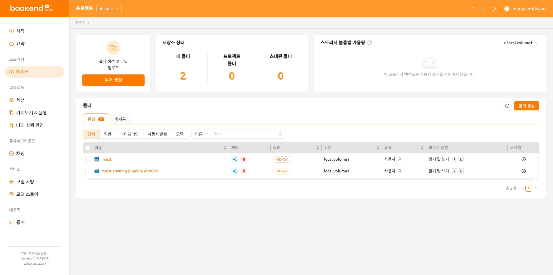
    main(args)

After creating the model folder, upload the files below.

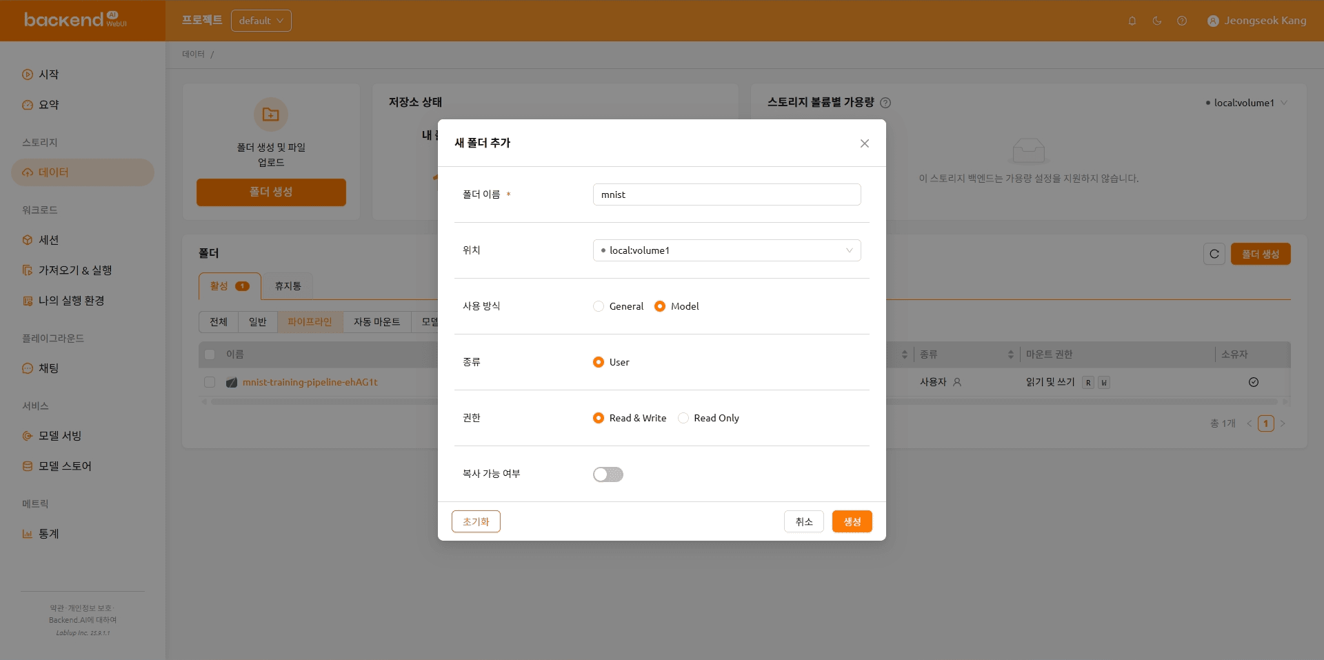Create a Model Folder

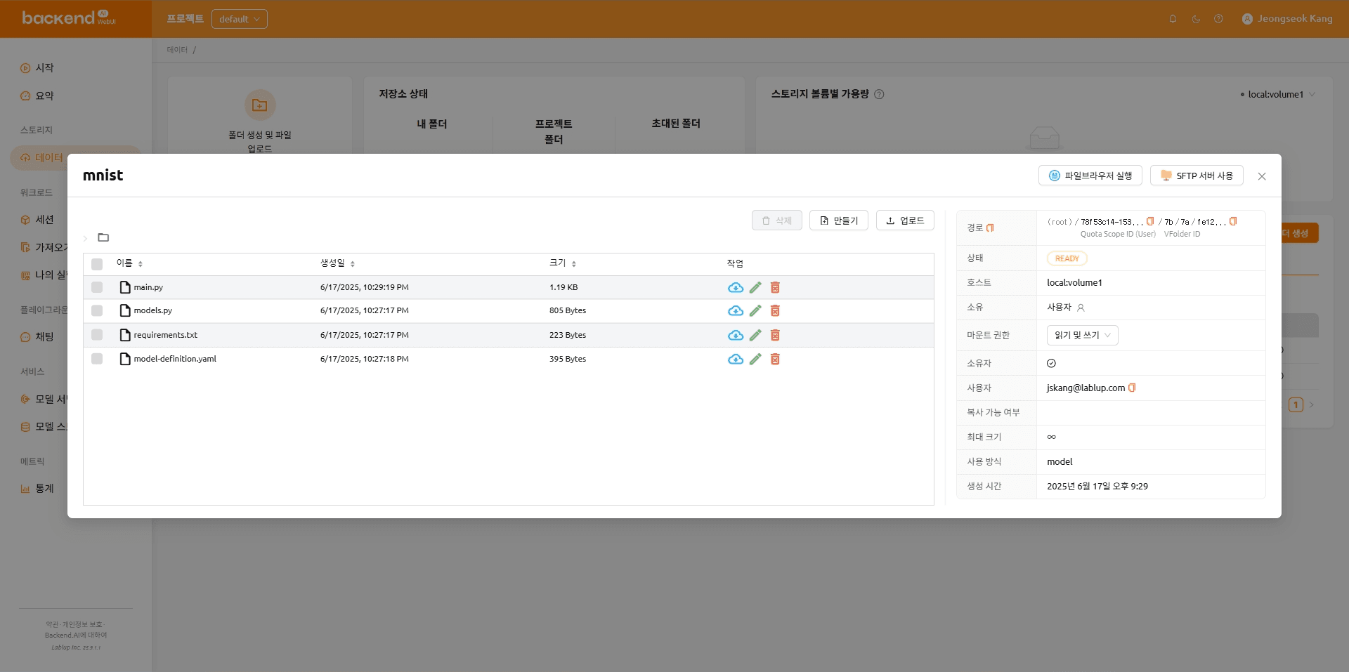
The folder organization after the files are uploaded is shown below.

mnist
    |---- main.py
    |---- models.py
    |---- requirements.txt
    \---- model-definition.yaml

import os
from http import HTTPStatus
from pathlib import Path

import gradio
import numpy as np
import torch
from fastapi import FastAPI, Response
from fastapi.responses import JSONResponse
from torchvision import transforms

from models import Net

CHECKPOINT_PATH = Path(os.getenv("CHECKPOINT_PATH")).joinpath(os.getenv("BACKENDAI_PIPELINE_JOB_ID", "mnist_cnn")).with_suffix(".ckpt")

model = Net()
model.load_state_dict(torch.load(CHECKPOINT_PATH))

transform = transforms.Compose([
    transforms.ToTensor(),
    transforms.Normalize((0.1307,), (0.3081,)),
    transforms.Grayscale(),
])

app = FastAPI()


@app.get("/health", status_code=HTTPStatus.OK)
async def health_check() -> Response:
    return JSONResponse({"healthy": True})


def fn(img: np.ndarray) -> int:
    x = transform(img).unsqueeze(0)  # Add batch dimension
    x = model(x)
    x = x.argmax(dim=1, keepdim=True)  # Get the index of the max log-probability
    return int(x.item())  # Convert tensor to int and return


gradio_app = gradio.Interface(
    fn=fn,
    inputs=["image"],
    outputs=["number"],
)

app = gradio.mount_gradio_app(app, gradio_app, path="/")

import torch
import torch.nn as nn
import torch.nn.functional as F


class Net(nn.Module):
    def __init__(self):
        super(Net, self).__init__()
        self.conv1 = nn.Conv2d(1, 32, 3, 1)
        self.conv2 = nn.Conv2d(32, 64, 3, 1)
        self.dropout1 = nn.Dropout(0.25)
        self.dropout2 = nn.Dropout(0.5)
        self.fc1 = nn.Linear(9216, 128)
        self.fc2 = nn.Linear(128, 10)

    def forward(self, x):
        x = self.conv1(x)
        x = F.relu(x)
        x = self.conv2(x)
        x = F.relu(x)
        x = F.max_pool2d(x, 2)
        x = self.dropout1(x)
        x = torch.flatten(x, 1)
        x = self.fc1(x)
        x = F.relu(x)
        x = self.dropout2(x)
        x = self.fc2(x)
        output = F.log_softmax(x, dim=1)
        return output

fastapi[standard]==0.115.12  # https://github.com/fastapi/fastapi
gradio==5.33.0  # https://github.com/gradio-app/gradio
torch==2.7.1  # https://github.com/pytorch/pytorch
torchvision==0.22.1  # https://github.com/pytorch/vision

models:
  - name: mnist-gradio-demo
    model_path: /models
    service:
      pre_start_actions:
        - action: run_command
          args:
            command: ["pip", "install", "-r", "/models/requirements.txt"]
      start_command:
        - fastapi
        - run
        - /models/main.py
      port: 8000
      health_check:
        path: /health
        max_retries: 5

Adding a task

Back in Backend.AI FastTrack 2, add tasks to the pipeline in order.

NOTE

You can drag and drop the desired task from the list of task templates as shown below. For more information, see the “Creating a task” topic in our previous blog. 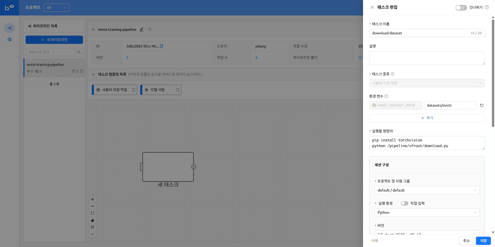Dragging tasks

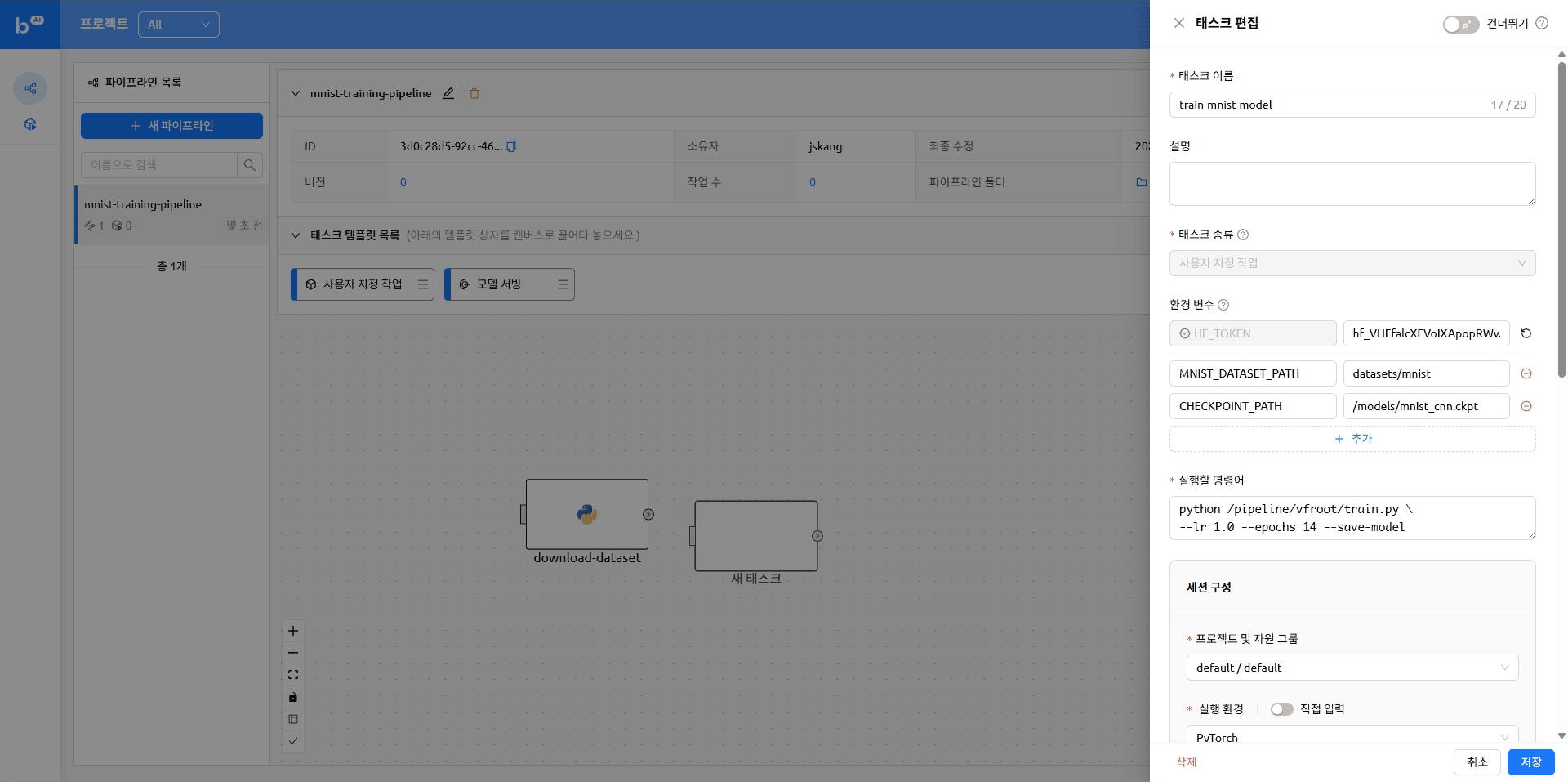
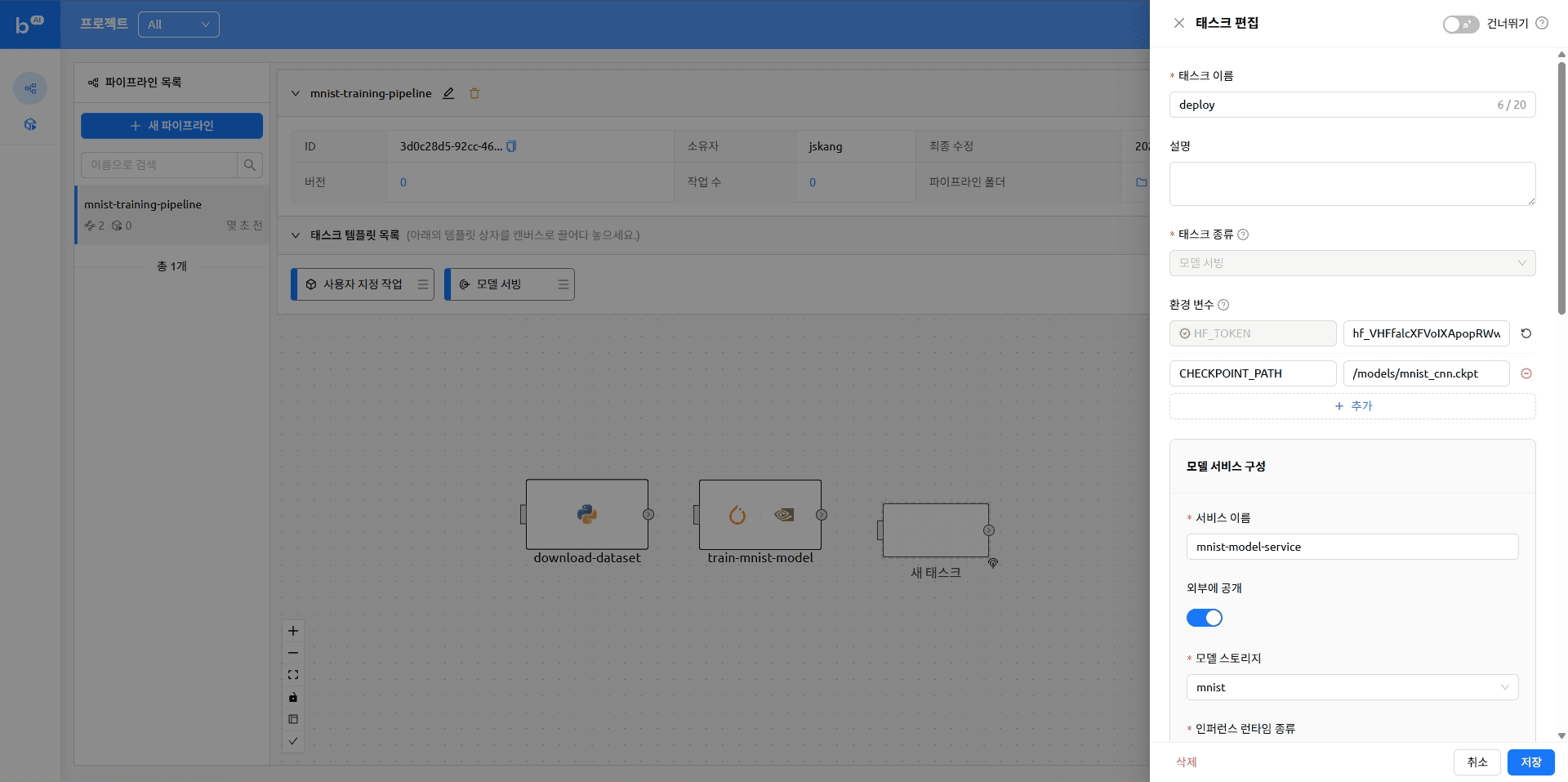
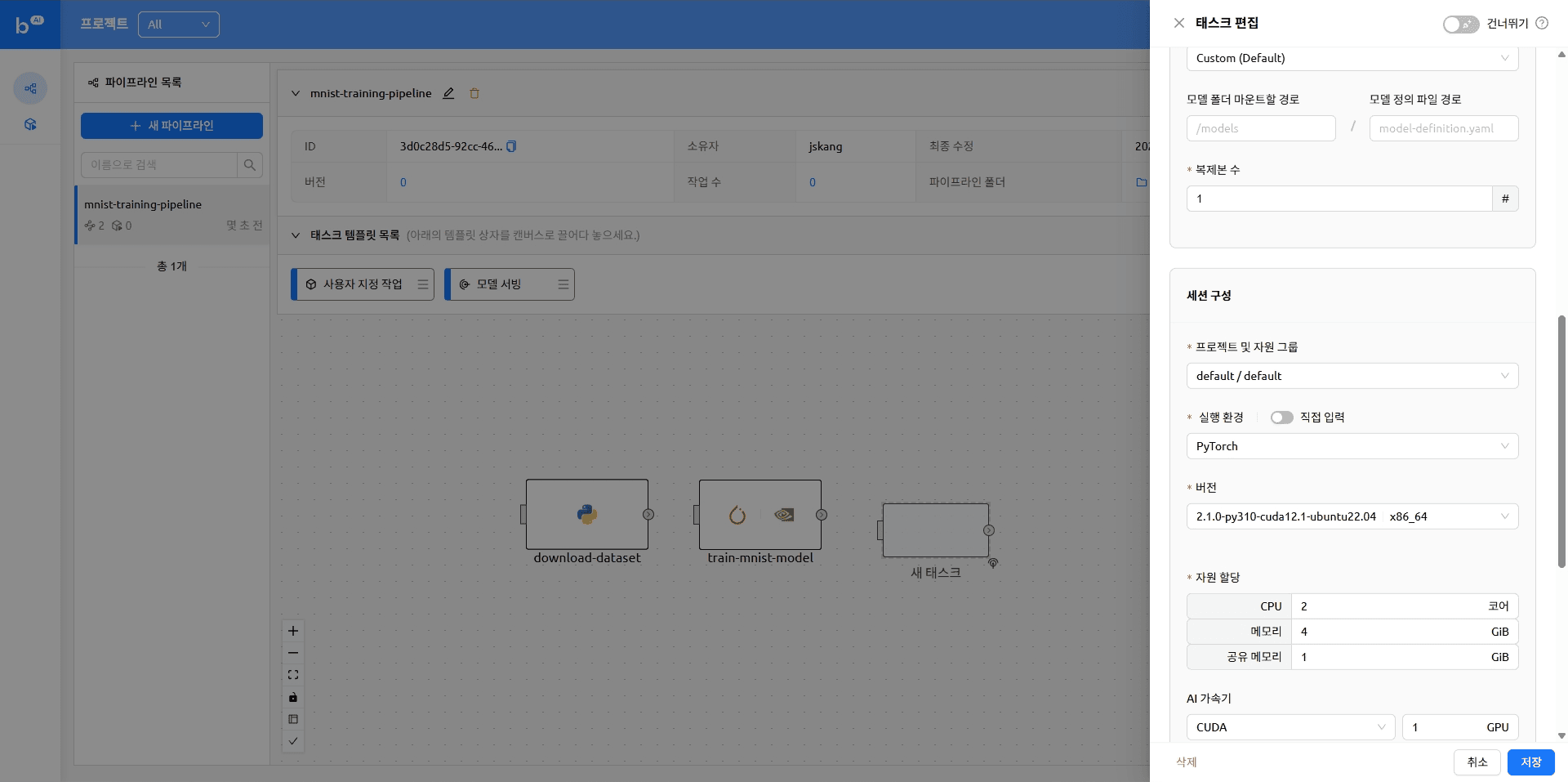
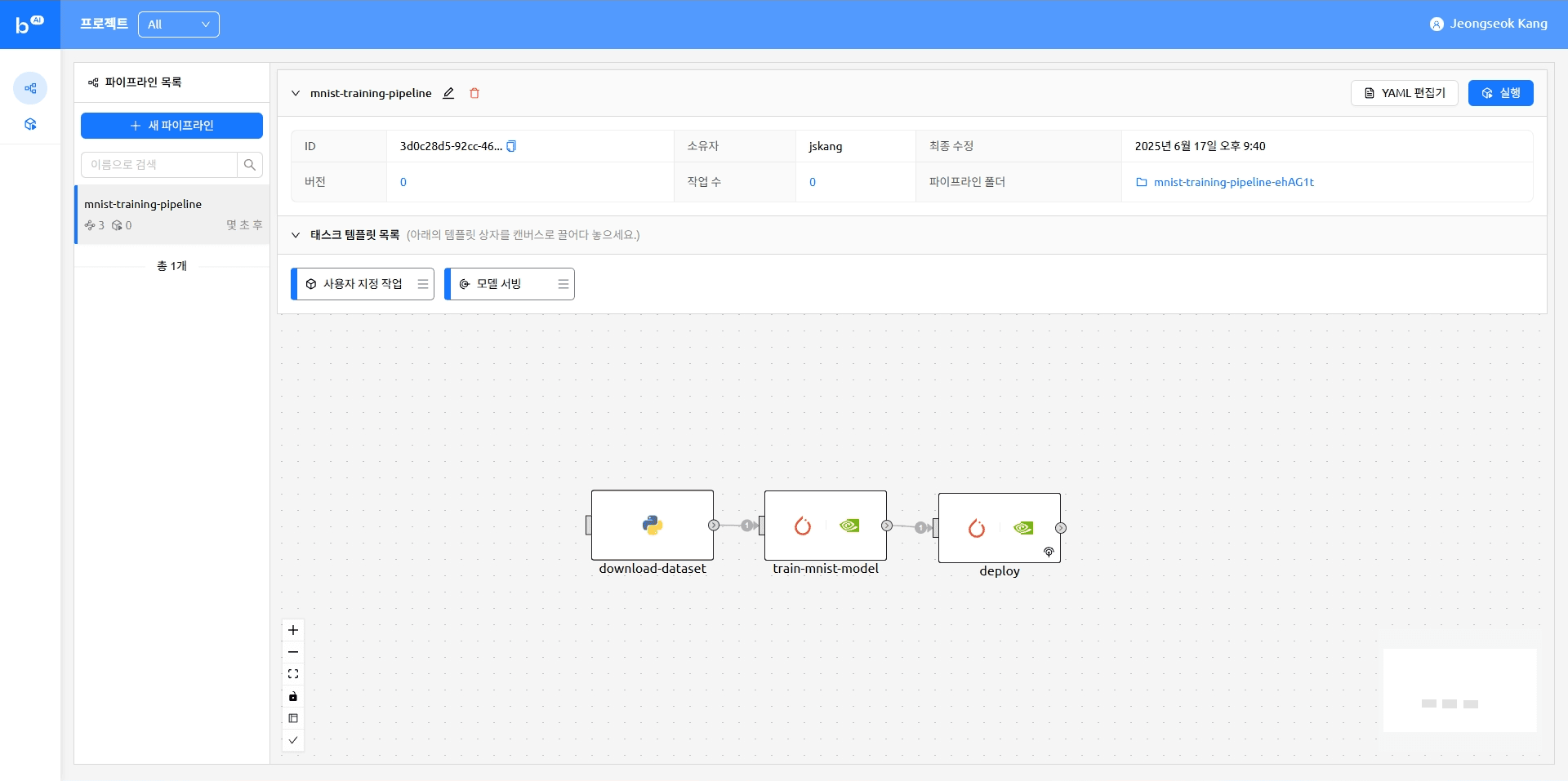
The pipeline with tasks added looks like this

version: 25.9.0
name: mnist-training-pipeline
description: ''
ownership:
  domain_name: default
  scope: user
environment:
  envs:
    HF_TOKEN: ****
tasks:
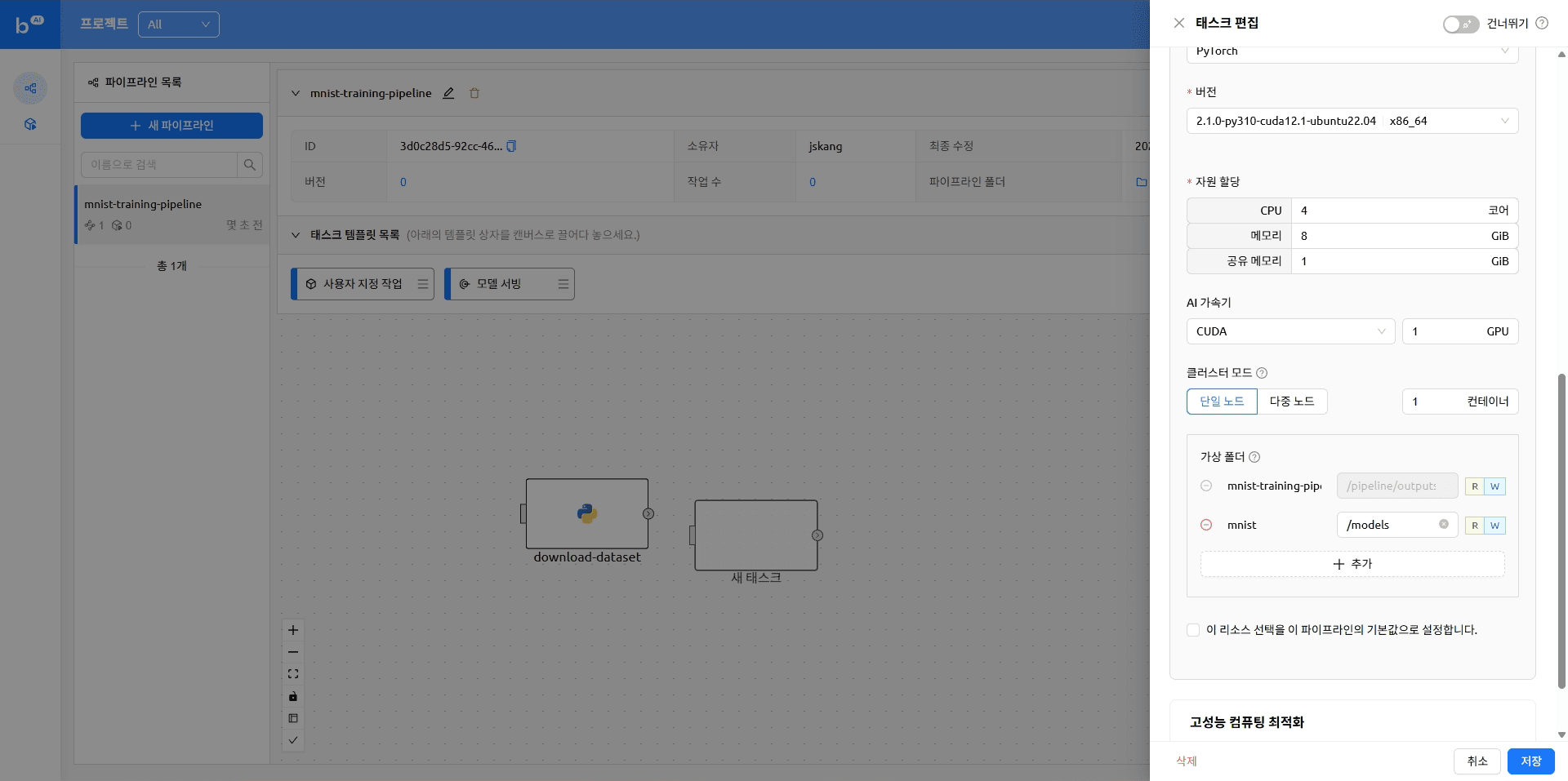
- name: train-mnist-model
  description: ''
  type: default
  cluster_mode: single-node
  cluster_size: 1
  module_uri: ''
  environment:
    project: default
    scaling-group: default
    image: cr.backend.ai/stable/python-pytorch:2.1.0-py310-cuda12.1-ubuntu22.04
    envs:
      MNIST_DATASET_PATH: datasets/mnist
      CHECKPOINT_PATH: /models/mnist_cnn.ckpt
  resources:
    cpu: 4
    mem: 4g
    cuda.device: '1'
  resource_opts:
    shmem: 0g
  dependencies:
  - download-dataset
  mounts:
  - mnist:/models
  skip: false
  command: python /pipeline/vfroot/mnist/train.py --lr 1.0 --epochs 14 --save-model
- name: download-dataset
  description: ''
  type: default
  cluster_mode: single-node
  cluster_size: 1
  module_uri: ''
  environment:
    project: default
    scaling-group: default
    image: cr.backend.ai/stable/python:3.9-ubuntu20.04
    envs:
      MNIST_DATASET_PATH: datasets/mnist
  resources:
    cpu: 1
    mem: 4g
  resource_opts:
    shmem: 0g
  dependencies: []
  mounts: []
  skip: false
  command: 'pip install torchvision

    python /pipeline/vfroot/mnist/download.py'
- name: deploy
  description: ''
  type: serving
  cluster_mode: single-node
  cluster_size: 1
  module_uri: ''
  environment:
    project: default
    scaling-group: default
    image: cr.backend.ai/stable/python-pytorch:2.1.0-py310-cuda12.1-ubuntu22.04
    envs: {}
  resources:
    cpu: 2
    mem: 4g
    cuda.device: '1'
  resource_opts:
    shmem: 0g
  dependencies:
  - train-mnist-model
  mounts: []
  skip: false
  service:
    name: mnist
    model: mnist
    model_mount_destination: /models
    runtime_variant: custom
    replicas: 1
    open_to_public: true

Running a Pipeline

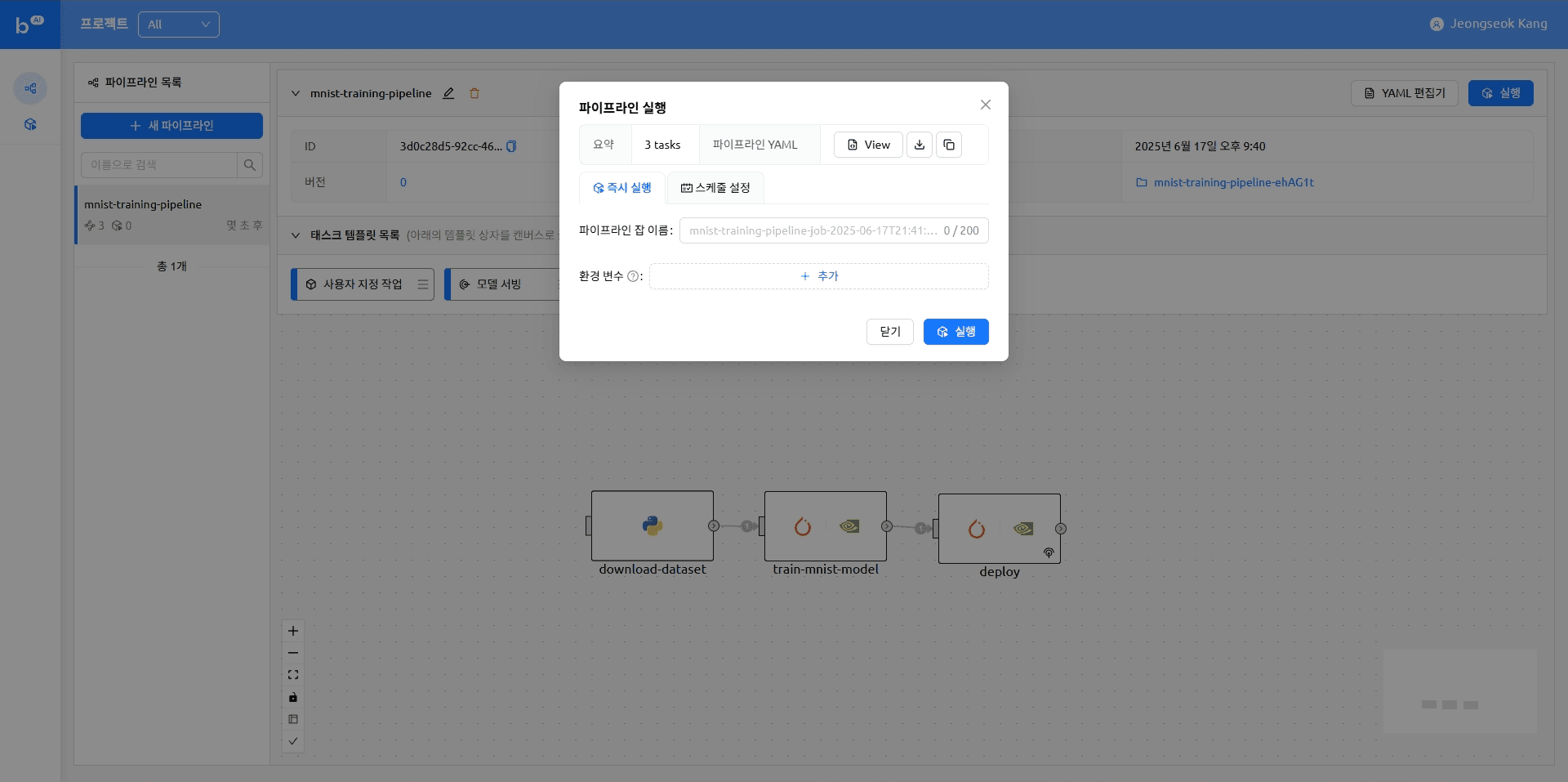
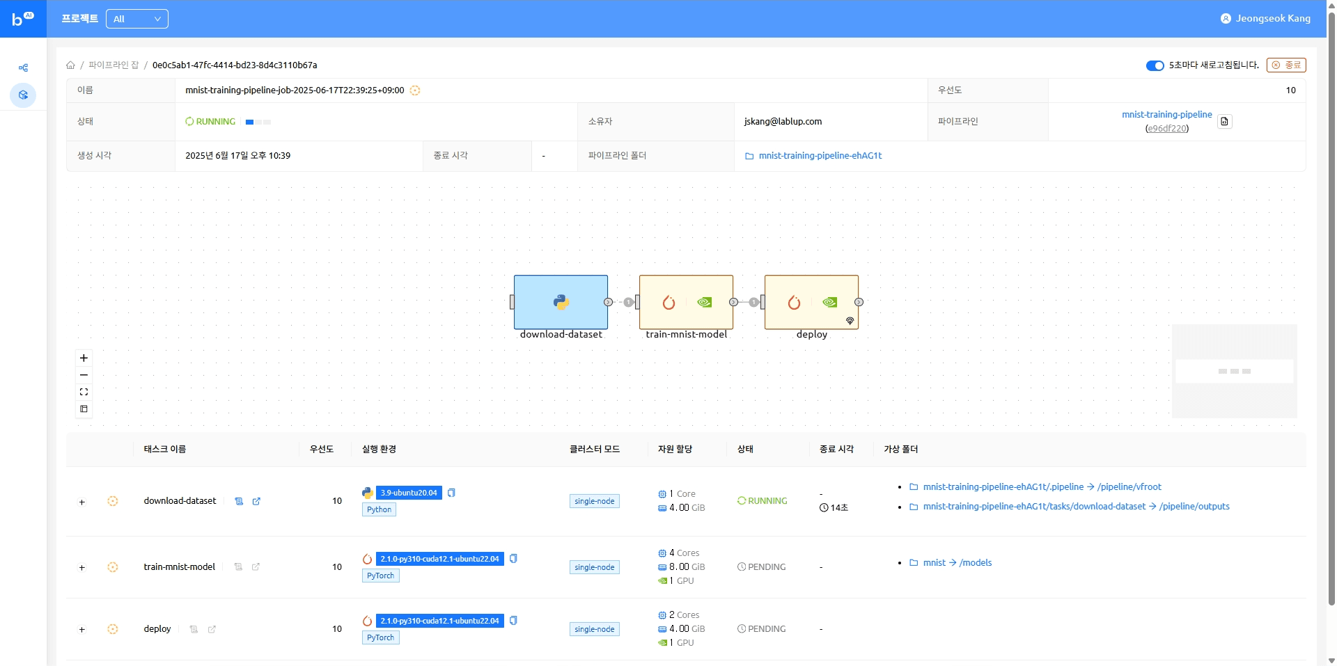
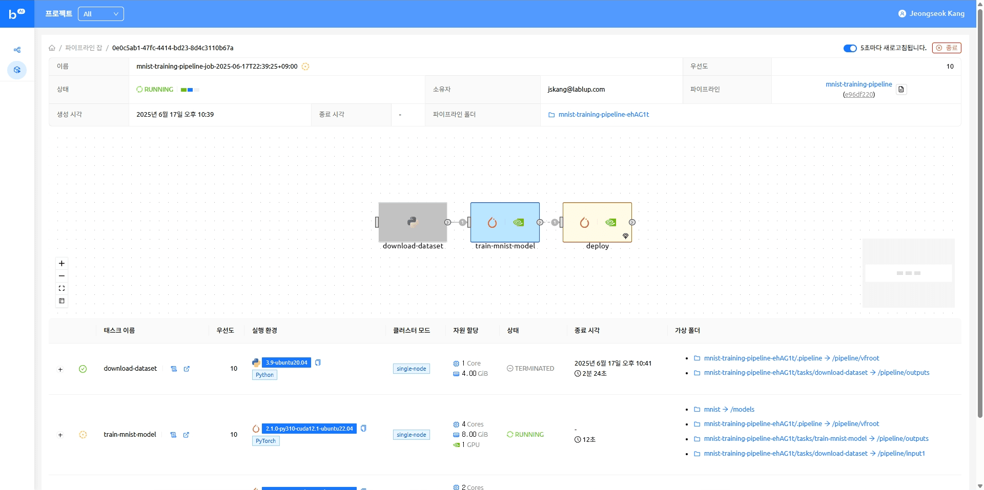
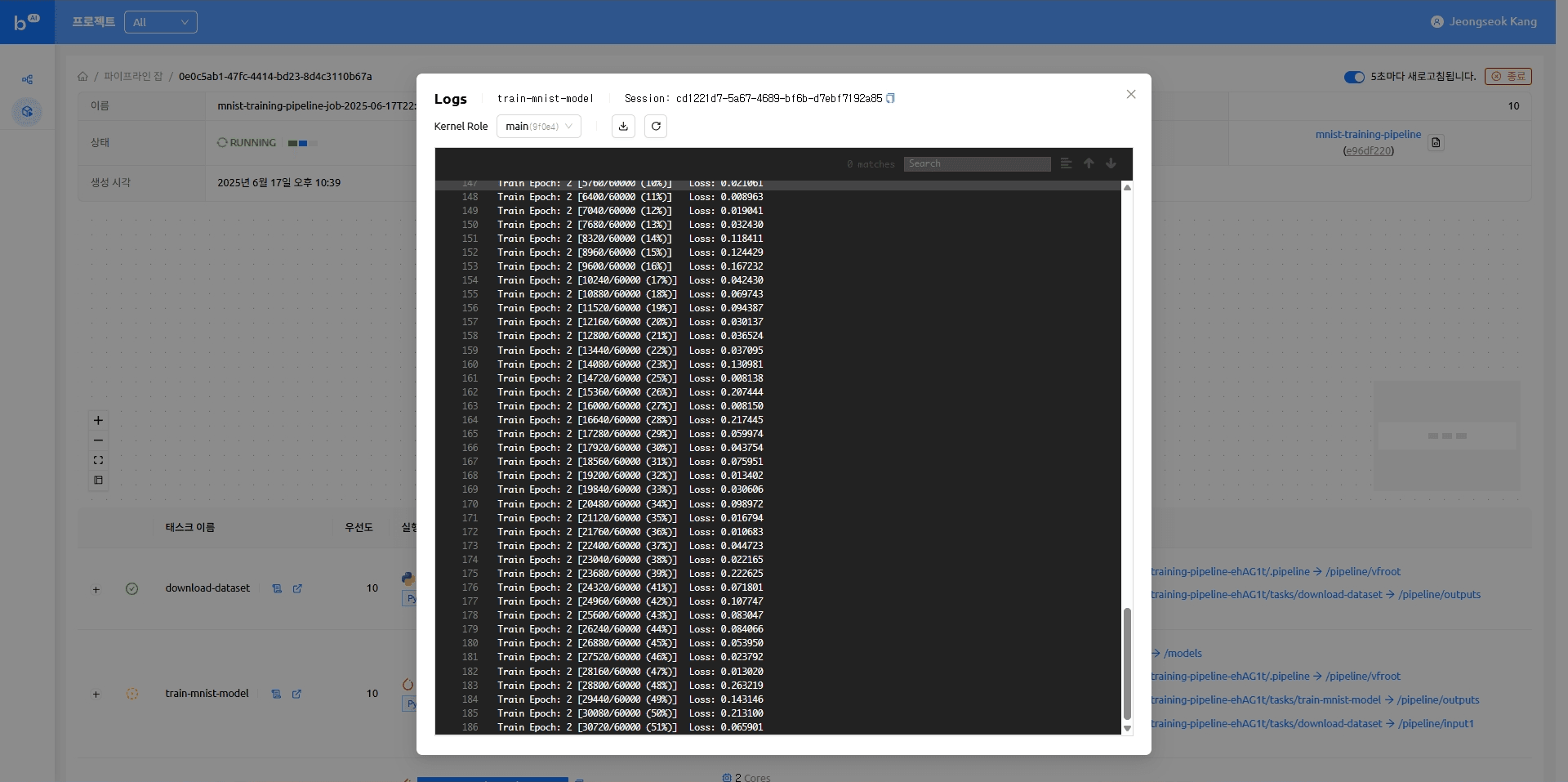
When the model serving task completes, the model appears as an accessible endpoint. Clicking that endpoint takes you to the Gradio demo page where you can try running model inference.

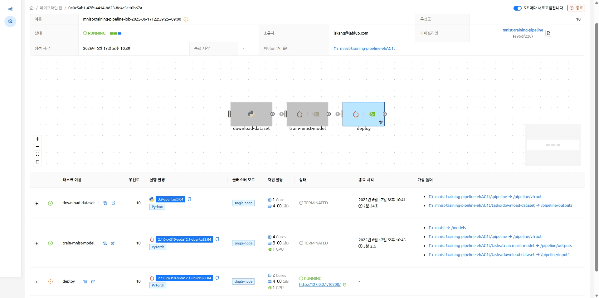The endpoint on which the MNIST model is running (http://127.0.0.1:10200)

Serving a Model

Upload some random MNIST data and run inference to see that the model trained well.

Closing

In this post, we showed you how to build a simple model training and serving pipeline using Backend.AI FastTrack 2. As always, we're always interested in hearing from machine learning researchers. If there's a topic you'd like to see us cover further, feel free to send us your thoughts at contact@lablup.com.

Thank You!

Appendix

MNIST Dataset

You can use the Python script below to convert a MNIST dataset file of the form MNIST/raw/t10k-images-idx3-ubyte to an image file.

import json
from pathlib import Path

import numpy as np
import matplotlib.pyplot as plt

root_path = Path(__file__).parent.parent

with open(root_path / "datasets/mnist/train/dataset_info.json", "r") as f:
    dataset_info = json.load(f)

image_size = 28
test_num_examples = dataset_info["splits"]["test"]["num_examples"]

with open(root_path / "datasets/mnist/MNIST/raw/t10k-images-idx3-ubyte", "rb") as f:
    f.read(16)  # Skip the header
    buf = f.read(image_size * image_size * test_num_examples)
data = np.frombuffer(buf, dtype=np.uint8).astype(np.float32)
data = data.reshape(test_num_examples, image_size, image_size)

for i in range(10):
    plt.imsave(root_path / f"datasets/{i}.png", data[i], cmap="gray")

Sculley, David, et al. "Hidden technical debt in machine learning systems." Advances in neural information processing systems 28 (2015). ↩
Jimmy Lin and Dmitriy Ryaboy. 2013. Scaling big data mining infrastructure: the twitter experience. SIGKDD Explor. Newsl. 14, 2 (December 2012), 6–19. https://doi.org/10.1145/2481244.2481247 ↩
D. Kreuzberger, N. Kühl and S. Hirschl, "Machine Learning Operations (MLOps): Overview, Definition, and Architecture," in IEEE Access, vol. 11, pp. 31866-31879, 2023, doi: 10.1109/ACCESS.2023.3262138. ↩
https://airflow.apache.org/ ↩
https://www.kubeflow.org/ ↩

Blog

Engineering

Backend.AI FastTrack 2 Guide for Airflow Users: Seamless Integration from Training to Serving

Backend.AI FastTrack 2 Guide for Airflow Users: Seamless Integration from Training to Serving

Why Do We Need Backend.AI FastTrack 2?

Reality: ML Code Is Just the Tip of the Iceberg

Limitations of Existing MLOps Tools

The Core Problem: Fragmented ML Workflows

The Solution: Backend.AI FastTrack 2 Model Serving

A True Ally for Researchers

Real-World Example: Migrating from Airflow to Backend.AI FastTrack 2

Airflow

Running and Initializing the Container

Creating a DAG

Backend.AI FastTrack 2

Creating a new pipeline

Uploading a file

Adding a task

Running a Pipeline

Serving a Model

Closing

Appendix

MNIST Dataset

Footnotes